Auto calculating a running balance…

Lets start with a little recap….

• you know your Total Combined Income
• you know how much you need to leave in General Expenses
• you know how much you are planning to transfer/allocate to other accounts
• you know what is left over to play with in the end
• you can see how much we have transferred into our different accounts

(and if you are not happy you know you can adjust one figure and all the rest will automatically adjust to reflect the change….aren’t you clever?)

What do we need to know now?

Well, we know that different amounts are expected to come out of our expense account at a future date and you have listed those expected bills already.

Go along and enter the amounts of the bills you are expecting, that is, when you expect them and what you expect them to be. The only way you will know if you have enough funds in the account to cover those expenses is by entering a formula which will allow you to keep a running balance.

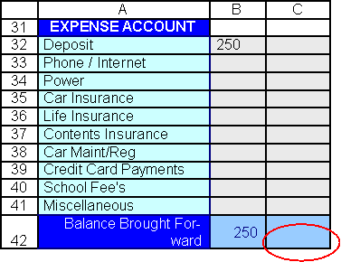
I will illustrate how to do this using the below example, remember your exact formula may be different:

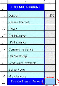
1. Click the cell next to the ‘balance brought forward’ field to highlight it
2. Enter the following formula  =(B32-B33-B34-B35-B36-B37-B38-B39-B40-B41)

Or in other words, the balance brought forward is the deposit, less whatever bill comes out.

Now in this case the next cell along on the balance brought forward (BFF) field will not be exactly that same as the first, so we cant just go ahead and drag the little solid square like before…as the formula in the rest of the BBF cells will actually include the balance of the first BBF cell, so now you need to enter a new formula.

1. Click the second empty cell to the right in the Balance Brought Forward field
2. Enter the following formula =(B42 +C32 -C33-C34-C35-C36-C37-C38-C39-C40-C41)…Or in other words, this new balance brought forward is the sum of the previous balance, plus the new deposit, less all the bills.
3. NOW you can drag this formula all the way to the end

Naturally the same method will apply with savings accounts.

Things to consider:

When setting up your savings account section you may want to consider having simply a DEPOSIT field, followed by an INTEREST earned field, and a WITHDRAWAL field. This way you can enter any bonus interest you earn, and also enter the occasions when you make a withdrawal in order to keep track of your savings.

And finally, by adding a last cell at the bottom of the spread sheet showing the total of ALL savings you will know at a glance what you have to draw on in an emergency. Remember the formula: this cell =(the cell references that you wish to add together)

Annual Totals

Now that you know the totals of all your income and expenses for each income and budget cycle, it will also be useful to see what your total annual expenditure is so that you can regularly review your overall financial management.

To do this the same method applies to total left to right rows as it does to calculate top to bottom columns.

Simply highlight the entire row, then using the Greek symbol ∑ you can immediately get the total spend for each particular area with one single click.

By now you pretty much know all there is to know about setting up your basic financial spreadsheet in Microsoft Excel. There is however one more thing you might find useful, and that is freezing panes. This is a handy thing to know because as you begin to use your spreadsheet each pay cycle you will gradually end up moving further and further to the right of your sheet and you will no longer be able to see the list on the left. By learning how to freeze sections of your spreadsheet you will be able to over come this by making it stick in one spot, effectively allowing your budget data to slide beneath the list on the left so that the list is always in view. If you want to learn how to do that, it’s quite simple, click here and I’ll show you. But if you don’t feel up to it just click here go straight to the end of the spreadsheet tutorials.

Time to get a little tricky, only a little…

Now it’s starting to get fun, it’s time to try a tiny bit of manual formulation.

Ask yourself, what do you need to know now? Well, naturally after you have decided to allocate funds here and there you will need to know how much you have left to play with.

• You know your Total Combined Income
• You know how much you need to leave in General Expenses
• You know how much you are planning to transfer/allocate to other accounts

So let’s see what’s left?

1. Click the empty cell directly next to ‘PLAY MONEY’ or whatever name you may have given that left over $$$ cell.
2. Now type the following =(B9-B26)

(Remember your cell references may differ but the process is the same) 

*THE FORMULA MUST BE IN BRACKETS AND MUST BEGIN WITH = 

What you are asking the spreadsheet to do is take away your total expenses from your total income……and asking, what is left?

Here is where you will find out if you need to adjust anything in order to make sure you really do have enough money without going into the red.

Don’t forget to copy that formula all the way along by clicking the cell, and dragging the solid black square all the way to the end.

Now we can sort out your other accounts.

Transfer data from one cell to another

Once again, what do you know so far?

• you know your Total Combined Income
• you know how much you need to leave in General Expenses
• you know how much you are planning to transfer/allocate to other accounts

AND

• Now you also know what is left over to play with in the end
• So now we will work out what is happening with the money you are transferring into your ‘expense account’ and any other accounts you may have included in your spreadsheet.

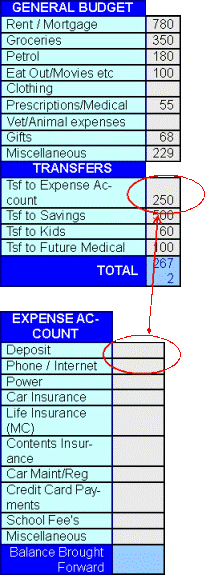
Remember we made the first cell under the heading of ‘EXPENSES’ into a deposit field. So we need to make the blank cell next to it automatically contain the same amount that we already allocated whilst in our general expenses section. So, Tsf to Expense = Deposit. The image on the right illustrates this function.

 

So it’s time to do another formula.

1. Click on the blank cell next to the deposit field
2. Enter the formula which tells the spreadsheet that you want the cell reference next to ‘deposit’ to = the same as the cell reference in which you entered the amount you intended to transfer into the expense account.

So for example: If the cell reference for ‘tsf to Expenses’ was B21 (that is, the amount you want to transfer from GENERAL BUDGET to EXPENSES), and the blank cell reference next to deposit in EXPENSES is B32 then the formula will read:

=(B32=B21) 

Or in other words….whatever you enter in B21 will automatically be transferred into B32 

Don’t forget to copy that formula all the way along by clicking the cell, and dragging the solid black square all the way to the end.

Do the same for any other accounts you have decided to transfer funds into.

If you have a field in GENERAL BUDGET that says you are going to transfer funds from general expenses to say, ‘savings’, then in the blank cell next to DEPOSIT, under the heading of ‘SAVINGS’ you need to enter the formula that says the two cells = the same.

NOTE

The same will not work in reverse. I.E. if you manually enter a figure into the actual expense account deposit section, it will not automatically change the transfer amount in GENERAL BUDGET…..think about it. That is not what the formula asks for.

So keep it simple and work from the GENERAL BUDGET section.

The next post will show you how to auto-calculate a running balance, click here to go there now.

Adding totals with a simple click…

What god is a spreadsheet if it doesn’t add up the totals for you, to set this function up is so easy. We’ll start with working out your income totals. But first we had better enter the income data.

Do you have the same income every time?

YES: Great, easy.

• Enter your income next to your name under the first date cell
• Click anywhere OUTSIDE that cell, this tells the spreadsheet you have finished entering data in that cell
• Now click on the cell again. Remember that solid square appearing in the bottom right corner? (We first saw it back when we were entering dates)
• Click on the solid square and drag it ALL THE WAY to the other end of your spreadsheet. I.E. where your dates end.

Woo Hoo! It’s all there for you. No need to type the same info again and again.

NO, My income changes all the time: No Problem.

You’ll just have to enter it as you earn. Of course, you can enter projected figures because you can change them ANY time you like.

BUT

If you have consistent income that differs due to shifts for example, like $500 one week, $540 the next, then the same rule applies as above. Enter the first amount in the first cell. Enter the second amount in the next cell along. Highlight them both, and then drag that little solid square all the way to the end.

Woo Hoo! It’s all there for you. No need to type the same info again and again.

Now that you have entered some income data, let’s add it up.

1. Highlight the figures in the first dated column all the way down to the empty cell next to Total Combined Income. Remember how? Click on the first income cell. Whilst holding the click, drag down all the way to and including the empty cell next to ‘Total Combined Income’.
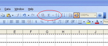
2. Release the click and move your cursor up to the tool bar again and look for a little Greek symbol: Looks like this:  ∑ Can you see it? Click it.

 

 

 

 

 

Another Woo Hoo as there in the totals cell  IS the total!

So easy, don’t you feel excited at how great you are doing?

Now I want to show you the formula that made your income all add up.

So, click on the cell that now has your Total Combined Income amount.

Look up to the white bar where all the text is displayed and you should see this formula:

=SUM(B5:B7) …..or similar

Huh! What does it mean? Well, its spreadsheet speak for

“this cell here equals the total sum of the amounts entered in the cells from B5 to B7”

The exciting thing here is that you could have entered the formula manually, but you didn’t have to. Don’t be disappointed. You’ll get the chance to do some manual formulations later, if you want to of course.

Now click on the cell that now has your total income amount in it. See that solid black square? Drag it along to the end of your spreadsheet and the same formula will automatically be copied all the way along so that your totals will always add up.

Now let’s get onto the totals of your General expenses…..

Well, as you have probably guessed, same as before.

Enter your general expenses alongside the cell that relates to the specific expense and under the date that you will be paying it.

If you refer back to the example I gave you of my spreadsheet you will see that this section is likely to be the things you pay directly out of your pay cheque, and occasional shopping spree’s etc. Not your regular bills.

Now do the Greek thing, highlight the column to the empty total general expenses cell and hit  ∑

And of course, you need to make that formula apply all the way along the spreadsheet. So click the first cell, click and drag the solid back square all the way along, and it’s done.

So So easy!

Wanna get a little more tricky? Are you feeling confident? Go on, click here to learn a little more…